gender <- c("female", "female", "male", "female", "male", "male")
height <- c(168, 165, 193, 165, 179, 180)
exercise <- c(180, 60, 150, 280, 90, 200)12 Working with Dataframes
Dataframes
Dataframes group a collection of related vectors. They are like Excel files, but with certain rules:
- The rows are observations.
- The columns are variables and have names.
- All columns must be the same length.
12.1 Create a dataframe
survey <- data.frame(gender, height, exercise)
survey
gender height exercise
1 female 168 180
2 female 165 60
3 male 193 150
4 female 165 280
5 male 179 90
6 male 180 20012.2 Check the dataframe
View(survey)Caution: Do NOT use the View() function for large datasets. It is best to use for small datasets such as this one.
12.3 Plot the data
plot(survey)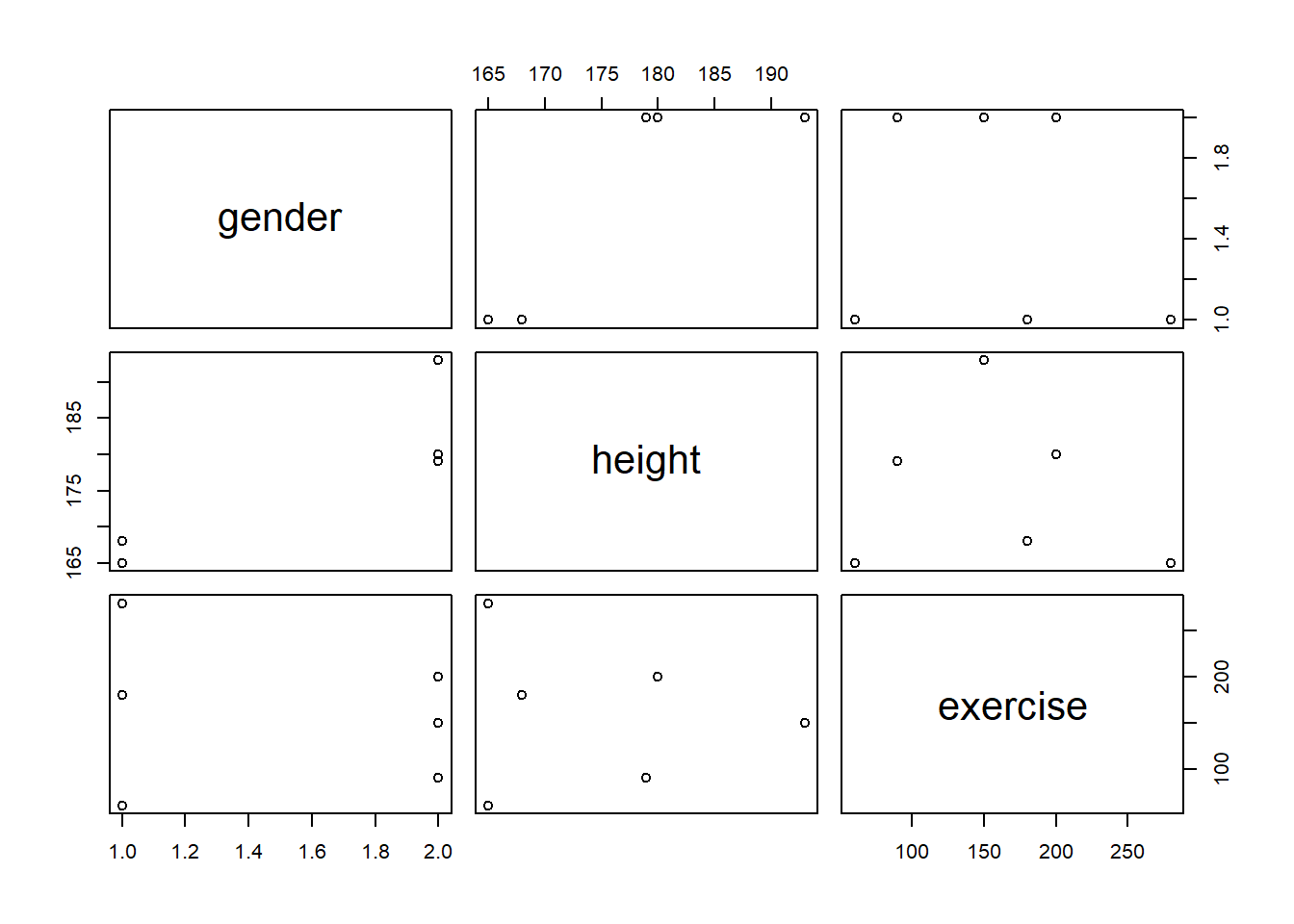
12.4 Working with dataframes
View the column names and structures:
str(survey)'data.frame': 6 obs. of 3 variables:
$ gender : chr "female" "female" "male" "female" ...
$ height : num 168 165 193 165 179 180
$ exercise: num 180 60 150 280 90 200Extract columns:
survey$height # the $ is the most common way to extract columns[1] 168 165 193 165 179 180survey[,2] # can also be done this way[1] 168 165 193 165 179 180survey[,2:3] # to extract multiple columns height exercise
1 168 180
2 165 60
3 193 150
4 165 280
5 179 90
6 180 200Extract rows:
survey[2,] gender height exercise
2 female 165 60survey[4:6,] # to extract multiple rows gender height exercise
4 female 165 280
5 male 179 90
6 male 180 200Add new rows:
survey2 <- rbind(survey, c("female", 166, 150), c("female", 165, 90))
survey2
gender height exercise
1 female 168 180
2 female 165 60
3 male 193 150
4 female 165 280
5 male 179 90
6 male 180 200
7 female 166 150
8 female 165 90Add new columns:
age <- c(19, 17, 17, 18, 18, 19, 18, 18)
survey2$age <- age
survey2
gender height exercise age
1 female 168 180 19
2 female 165 60 17
3 male 193 150 17
4 female 165 280 18
5 male 179 90 18
6 male 180 200 19
7 female 166 150 18
8 female 165 90 18Remove rows:
survey3 <- survey2[-c(4, 5), ] # removes rows 4 and 5 (notice the -)
survey3
gender height exercise age
1 female 168 180 19
2 female 165 60 17
3 male 193 150 17
6 male 180 200 19
7 female 166 150 18
8 female 165 90 18Remove columns:
survey4 <- survey3[,-3] # removes column 3 (exercise)
survey4
gender height age
1 female 168 19
2 female 165 17
3 male 193 17
6 male 180 19
7 female 166 18
8 female 165 18Accessing and changing column names:
colnames(survey4)[1] "gender" "height" "age" colnames(survey4) <- c("gender", "height.cm", "age")
survey4 gender height.cm age
1 female 168 19
2 female 165 17
3 male 193 17
6 male 180 19
7 female 166 18
8 female 165 1812.5 Save your revised data!
It is very important that you save all your changes made to your data otherwise you will need to run your code again! (Just like we did using Python!)
Use the write.csv() function to create and save a new csv file to your working directory. (Make sure your working directory is set so that it saves in that file.)
write.csv(survey4, "surveydata.csv")- For future R sessions, simply import the new csv file using read.csv() that you saved with all the changes.
12.6 Import your csv file
new.survey <- read.csv("surveydata.csv")
new.survey
X gender height.cm age
1 1 female 168 19
2 2 female 165 17
3 3 male 193 17
4 6 male 180 19
5 7 female 166 18
6 8 female 165 1812.7 Working with R data sets
R has several built-in data sets. Why?
A classic R dataset is the historical mtcars.
12.8 R documentation
Run the following for details about the data set:
> ?mtcars
12.9 mtcars data set
                     mpg cyl  disp  hp drat    wt  qsec vs am gear carb
Mazda RX4           21.0   6 160.0 110 3.90 2.620 16.46  0  1    4    4
Mazda RX4 Wag       21.0   6 160.0 110 3.90 2.875 17.02  0  1    4    4
Datsun 710          22.8   4 108.0  93 3.85 2.320 18.61  1  1    4    1
Hornet 4 Drive      21.4   6 258.0 110 3.08 3.215 19.44  1  0    3    1
Hornet Sportabout   18.7   8 360.0 175 3.15 3.440 17.02  0  0    3    2
Valiant             18.1   6 225.0 105 2.76 3.460 20.22  1  0    3    1
Duster 360          14.3   8 360.0 245 3.21 3.570 15.84  0  0    3    4
Merc 240D           24.4   4 146.7  62 3.69 3.190 20.00  1  0    4    2
Merc 230            22.8   4 140.8  95 3.92 3.150 22.90  1  0    4    2
Merc 280            19.2   6 167.6 123 3.92 3.440 18.30  1  0    4    4
Merc 280C           17.8   6 167.6 123 3.92 3.440 18.90  1  0    4    4
Merc 450SE          16.4   8 275.8 180 3.07 4.070 17.40  0  0    3    3
Merc 450SL          17.3   8 275.8 180 3.07 3.730 17.60  0  0    3    3
Merc 450SLC         15.2   8 275.8 180 3.07 3.780 18.00  0  0    3    3
Cadillac Fleetwood  10.4   8 472.0 205 2.93 5.250 17.98  0  0    3    4
Lincoln Continental 10.4   8 460.0 215 3.00 5.424 17.82  0  0    3    4
Chrysler Imperial   14.7   8 440.0 230 3.23 5.345 17.42  0  0    3    4
Fiat 128            32.4   4  78.7  66 4.08 2.200 19.47  1  1    4    1
Honda Civic         30.4   4  75.7  52 4.93 1.615 18.52  1  1    4    2
Toyota Corolla      33.9   4  71.1  65 4.22 1.835 19.90  1  1    4    1
Toyota Corona       21.5   4 120.1  97 3.70 2.465 20.01  1  0    3    1
Dodge Challenger    15.5   8 318.0 150 2.76 3.520 16.87  0  0    3    2
AMC Javelin         15.2   8 304.0 150 3.15 3.435 17.30  0  0    3    2
Camaro Z28          13.3   8 350.0 245 3.73 3.840 15.41  0  0    3    4
Pontiac Firebird    19.2   8 400.0 175 3.08 3.845 17.05  0  0    3    2
Fiat X1-9           27.3   4  79.0  66 4.08 1.935 18.90  1  1    4    1
Porsche 914-2       26.0   4 120.3  91 4.43 2.140 16.70  0  1    5    2
Lotus Europa        30.4   4  95.1 113 3.77 1.513 16.90  1  1    5    2
Ford Pantera L      15.8   8 351.0 264 4.22 3.170 14.50  0  1    5    4
Ferrari Dino        19.7   6 145.0 175 3.62 2.770 15.50  0  1    5    6
Maserati Bora       15.0   8 301.0 335 3.54 3.570 14.60  0  1    5    8
Volvo 142E          21.4   4 121.0 109 4.11 2.780 18.60  1  1    4    2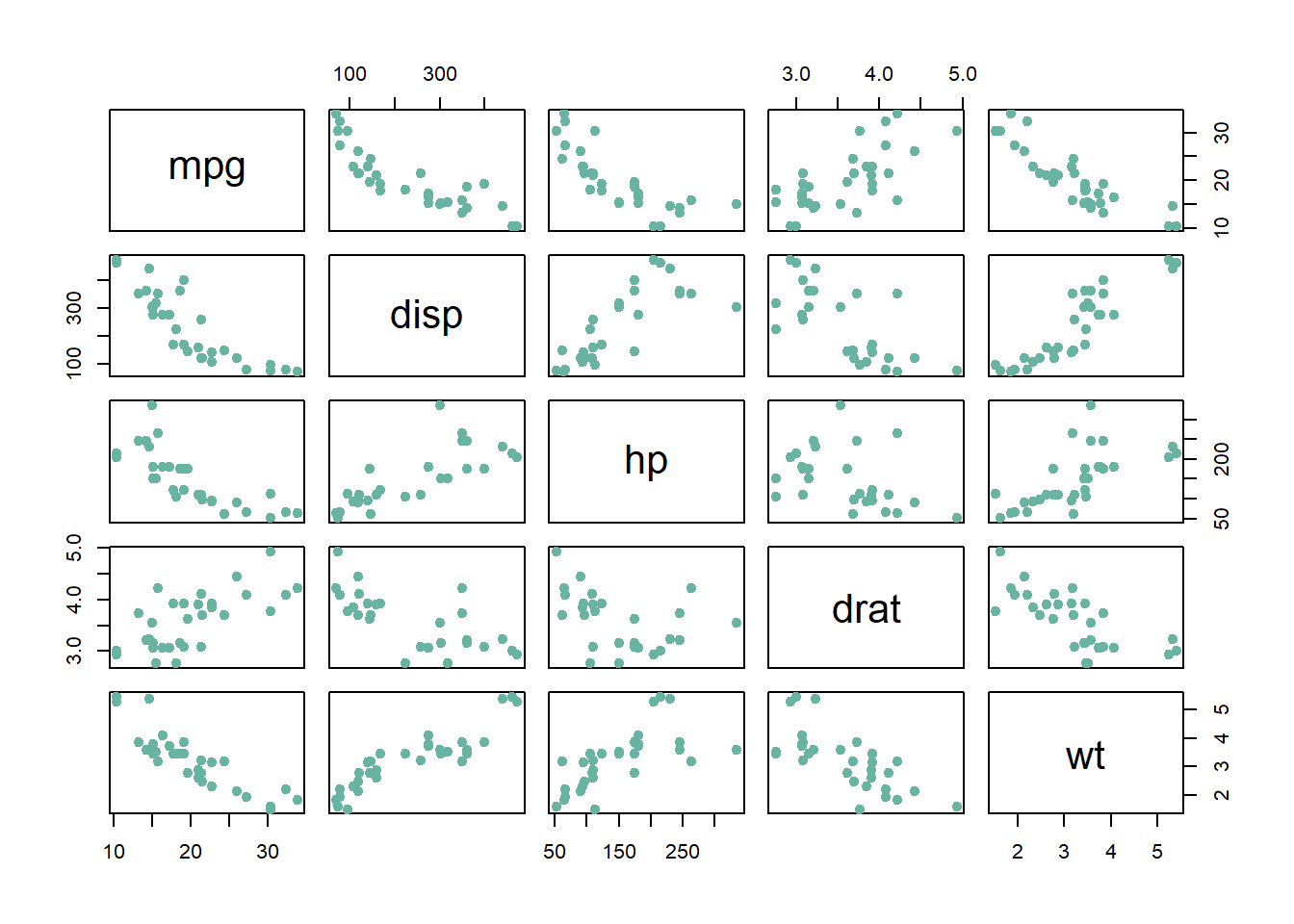
12.10 Common functions for data analysis
dim(mtcars)[1] 32 11summary(mtcars) mpg cyl disp hp
Min. :10.40 Min. :4.000 Min. : 71.1 Min. : 52.0
1st Qu.:15.43 1st Qu.:4.000 1st Qu.:120.8 1st Qu.: 96.5
Median :19.20 Median :6.000 Median :196.3 Median :123.0
Mean :20.09 Mean :6.188 Mean :230.7 Mean :146.7
3rd Qu.:22.80 3rd Qu.:8.000 3rd Qu.:326.0 3rd Qu.:180.0
Max. :33.90 Max. :8.000 Max. :472.0 Max. :335.0
drat wt qsec vs
Min. :2.760 Min. :1.513 Min. :14.50 Min. :0.0000
1st Qu.:3.080 1st Qu.:2.581 1st Qu.:16.89 1st Qu.:0.0000
Median :3.695 Median :3.325 Median :17.71 Median :0.0000
Mean :3.597 Mean :3.217 Mean :17.85 Mean :0.4375
3rd Qu.:3.920 3rd Qu.:3.610 3rd Qu.:18.90 3rd Qu.:1.0000
Max. :4.930 Max. :5.424 Max. :22.90 Max. :1.0000
am gear carb
Min. :0.0000 Min. :3.000 Min. :1.000
1st Qu.:0.0000 1st Qu.:3.000 1st Qu.:2.000
Median :0.0000 Median :4.000 Median :2.000
Mean :0.4062 Mean :3.688 Mean :2.812
3rd Qu.:1.0000 3rd Qu.:4.000 3rd Qu.:4.000
Max. :1.0000 Max. :5.000 Max. :8.000 12.11 The aggregate() function
We can create pivot tables:
aggregate(mtcars$mpg, by=list(mtcars$cyl), FUN=sum) Group.1 x
1 4 293.3
2 6 138.2
3 8 211.4aggregate(mtcars$mpg, by=list(mtcars$cyl), FUN=mean) Group.1 x
1 4 26.66364
2 6 19.74286
3 8 15.1000012.12 Correlation analysis
We can select the numeric variables and study the correlations between them. Correlation is a number between -1 (strong negative association) to +1 (strong positive association). A correlation of 0 means there is no correlation.
Let’s take a look at the correlations:
Code
num.vars <- mtcars[ , c(1,3:6)]
print(cor(num.vars))
mpg disp hp drat wt
mpg 1.0000000 -0.8475514 -0.7761684 0.6811719 -0.8676594
disp -0.8475514 1.0000000 0.7909486 -0.7102139 0.8879799
hp -0.7761684 0.7909486 1.0000000 -0.4487591 0.6587479
drat 0.6811719 -0.7102139 -0.4487591 1.0000000 -0.7124406
wt -0.8676594 0.8879799 0.6587479 -0.7124406 1.000000012.13 The apply() function
We can calculate summary statistics simultaneously for mutliple columns:
a1 <- apply(num.vars, 2, FUN = mean)
a1
mpg disp hp drat wt
20.090625 230.721875 146.687500 3.596563 3.217250 a1 <- apply(num.vars, 2, FUN = median)
a1 mpg disp hp drat wt
19.200 196.300 123.000 3.695 3.325 a1 <- apply(num.vars, 2, FUN = sd)
a1 mpg disp hp drat wt
6.0269481 123.9386938 68.5628685 0.5346787 0.9784574 12.14 Reflection questions
Reflection Questions
Why do all columns in a dataframe need to be the same length?
When is it appropriate to use View() to inspect a dataframe, and when should you avoid it?
How can visualizing data early in the analysis process help you detect issues or trends?
What are two different ways to extract a column from a dataframe? Which one do you find easier to remember?
What is the difference between rbind() and cbind() (or $ when adding columns)?
Why should you save your modified data to a file after making changes?
What would happen if you forgot to set the working directory before using write.csv()?
How can reading the documentation for a dataset (e.g., ?mtcars) improve your analysis?
What’s the difference between summary() and dim()? What does each tell you?
How can aggregate() be used to create pivot-table-like summaries in R?
What does it mean if the correlation between two variables is close to 1? What about close to 0?
What is the benefit of using apply() instead of writing separate commands for each column?
12.15 Exercises
Exercises
What are the three rules for data frames in R? Why are they important when working with real-world datasets (like survey results)?
You receive a CSV of customer feedback with 1,000 rows. A teammate stacked two rating columns side-by-side but one column has 999 entries. Explain exactly which tidy data-frame rule is being violated and what error this can cause when you try to bind columns.
Sam’s department receives a weekly CSV and wants to sanity-check it quickly. Explain how dim(x) and summary(x) together can reveal both structural and content anomalies.
Explain the issue with the following code and correct it.
df <- data.frame(
  name = c("Ana","Ben","Cal"),
  score = c(90, 85),
  passed = c(TRUE, TRUE, TRUE)
)
Why should you be careful using View()?
John wants the revenue vector but encounters an error. How can he fix it?
sales <- data.frame(store=c("A","B"), revenue=c(100,120))
x <- sales["revenue"]
mean(x)
For questions 7 to 12, create a data frame called bakery with columns month, cookies_sold, and cakes_sold for three months of data.
Amy wants only the cakes_sold column. Write three different ways to extract it as a vector.
Now Amy only wants to see February’s data, and then find all months where more than 130 cookies were sold.
Add a row for April where the bakery sold 170 cookies and 60 cakes.
Assume cookies sell for $2 each and cakes sell for $10 each. Add a revenue column in two different ways.
Amy accidentally entered April twice. Remove the 4th row from bakery.
Amy wants the names of the columns to be more professional: Month, Cookies, Cakes, and Revenue. Change them all at once.
Open the built-in dataset mtcars. Use head() to preview it and ? to learn more. Why are built-in datasets useful for practice?
What do dim() and summary() tell you about mtcars? Run them and interpret the results.
Rei typed the following code and got an error. Why does this happen, and how can she fix it?
mtcars[ , mpg] Monica wants the average miles per gallon (mpg) by number of cylinders (cyl). Use aggregate() to calculate this.
Adrian wants the average horsepower (hp) grouped by both cyl and gear. How can this be coded?
What does correlation measure? Calculate the correlation between mpg and hp in mtcars.
Find correlations among mpg, hp, and wt. Which two variables do you expect to be most negatively correlated?
Fatima wants the mean of each numeric column in mtcars. Use apply() to do this.
See below the following data frame:
scores <- data.frame(A = c(10,20,30), B = c(5,10,15))Use apply() to calculate each row’s sum.
- Ryan tried:
apply(mtcars, 2, summary)