# Import the dataset
customer_sales <- read.csv("BusinessMetrics.csv")13 Importing, Exploring, and Creating Data
13.1 Importing csv files
If you have an Excel file, it is easier to convert to a csv (comma deliminated) file.
Make sure the spreadsheet has been prepared. The top row is for the name of each variable, and every column MUST be the same length. Otherwise, the file will be read in as a list or some other structure type.
13.2 Import the dataset to your R session
What can you discover about the dataset?
13.3 Preliminary data exploration
dim(customer_sales)[1] 50 5summary(customer_sales) Product.Category Purchase.Amount Customer.Satisfaction.Rating
Length:50 Min. : 28.6 Min. :1.0
Class :character 1st Qu.:375.0 1st Qu.:2.0
Mode :character Median :572.6 Median :3.0
Mean :542.6 Mean :3.2
3rd Qu.:761.9 3rd Qu.:4.0
Max. :978.8 Max. :5.0
Repeat.Customer Previous.Purchase.Amount
Length:50 Min. : 0.0
Class :character 1st Qu.: 0.0
Mode :character Median :136.8
Mean :278.3
3rd Qu.:478.9
Max. :982.8 13.4 Installing R packages
Go to Help for CRAN packages search options.
Install the package.
You must run library(“name of package”) for each new R session.
13.5 Introducing the ‘dplyr’ package
Let’s try installing the R package commonly used for data manipulation:
# Remove the # symbol and install the package
#install.packages('dplyr')
⏳ Installation Tip
Wait for it!
Some packages take a while to install!
You only need to install a package once, but you will need to attach the library for each new R session.
library('dplyr')
Attaching package: 'dplyr'The following objects are masked from 'package:stats':
filter, lagThe following objects are masked from 'package:base':
intersect, setdiff, setequal, union13.6 Core functions in dplyr
select():
Choose specific columns from a data frame.
customer_sales_selected <- customer_sales %>%
  select(Purchase.Amount, Repeat.Customer)
   Purchase.Amount Repeat.Customer
1           553.33             Yes
2           718.04              No
3           606.74             Yes
4           549.43             Yes
5           429.42             Yes
6           649.44              No
7           443.21             Yes
8           892.86              No
9           964.03             Yes
10          389.61              No
11          793.81             Yes
12          533.61             Yes
13          572.36             Yes
14          926.34             Yes
15           80.33             Yes
16           96.26              No
17           30.02             Yes
18          834.29             Yes
19          780.38              No
20          871.31             Yes
21          978.83             Yes
22          801.17             Yes
23          466.86              No
24          782.72             Yes
25          127.09             Yes
26          643.52              No
27          151.92             Yes
28          945.22              No
29          526.63             Yes
30          420.52             Yes
31          271.91              No
32          776.49              No
33          461.59             Yes
34          572.75             Yes
35           28.60             Yes
36          621.46              No
37          615.97              No
38          620.76             Yes
39          944.31             Yes
40          685.00             Yes
41          365.91             Yes
42          442.66             Yes
43          700.65              No
44           69.62             Yes
45          670.10              No
46          673.93             Yes
47          218.28             Yes
48          137.64             Yes
49          322.27              No
50          370.07              No
filter():
Subset rows based on conditions.
customer_sales_filtered <- customer_sales %>%
  filter(Purchase.Amount > 550)
customer_sales_filtered Product.Category Purchase.Amount Customer.Satisfaction.Rating
1 Clothing 553.33 2
2 Clothing 718.04 3
3 Electronics 606.74 5
4 Sports 649.44 5
5 Clothing 892.86 4
6 Electronics 964.03 5
7 Clothing 793.81 5
8 Automotive 572.36 5
9 Sports 926.34 4
10 Clothing 834.29 2
11 Electronics 780.38 4
12 Automotive 871.31 1
13 Automotive 978.83 1
14 Automotive 801.17 2
15 Sports 782.72 5
16 Electronics 643.52 1
17 Sports 945.22 3
18 Automotive 776.49 1
19 Sports 572.75 3
20 Home Goods 621.46 3
21 Electronics 615.97 4
22 Home Goods 620.76 3
23 Clothing 944.31 2
24 Sports 685.00 3
25 Home Goods 700.65 4
26 Automotive 670.10 4
27 Home Goods 673.93 5
Repeat.Customer Previous.Purchase.Amount
1 Yes 125.04
2 No 0.00
3 Yes 417.70
4 No 0.00
5 No 0.00
6 Yes 663.07
7 Yes 238.23
8 Yes 622.62
9 Yes 480.12
10 Yes 389.63
11 No 0.00
12 Yes 879.67
13 Yes 111.83
14 Yes 101.45
15 Yes 556.30
16 No 0.00
17 No 0.00
18 No 0.00
19 Yes 453.45
20 No 0.00
21 No 0.00
22 Yes 842.73
23 Yes 905.60
24 Yes 47.18
25 No 0.00
26 No 0.00
27 Yes 148.57mutate():
Create new columns or modify existing ones.
For example, add a new column called Purchase.Amount.Tax:
customer_sales_mutated <- customer_sales %>%
  mutate(Purchase.Amount.Tax = Purchase.Amount * 0.15)
colnames(customer_sales_mutated)[1] "Product.Category" "Purchase.Amount"
[3] "Customer.Satisfaction.Rating" "Repeat.Customer"
[5] "Previous.Purchase.Amount" "Purchase.Amount.Tax" arrange():
Sort rows based on one or more columns.
For example, sort the dataset by Purchase.Amount in ascending order:
customer_sales_arranged <- customer_sales %>%
  arrange(Purchase.Amount)
customer_sales_arranged Product.Category Purchase.Amount Customer.Satisfaction.Rating
1 Automotive 28.60 4
2 Automotive 30.02 2
3 Electronics 69.62 3
4 Clothing 80.33 3
5 Clothing 96.26 1
6 Automotive 127.09 3
7 Sports 137.64 3
8 Clothing 151.92 4
9 Sports 218.28 2
10 Automotive 271.91 2
11 Sports 322.27 4
12 Sports 365.91 4
13 Automotive 370.07 2
14 Sports 389.61 5
15 Electronics 420.52 1
16 Home Goods 429.42 5
17 Electronics 442.66 4
18 Home Goods 443.21 5
19 Clothing 461.59 3
20 Clothing 466.86 3
21 Electronics 526.63 3
22 Electronics 533.61 1
23 Electronics 549.43 4
24 Clothing 553.33 2
25 Automotive 572.36 5
26 Sports 572.75 3
27 Electronics 606.74 5
28 Electronics 615.97 4
29 Home Goods 620.76 3
30 Home Goods 621.46 3
31 Electronics 643.52 1
32 Sports 649.44 5
33 Automotive 670.10 4
34 Home Goods 673.93 5
35 Sports 685.00 3
36 Home Goods 700.65 4
37 Clothing 718.04 3
38 Automotive 776.49 1
39 Electronics 780.38 4
40 Sports 782.72 5
41 Clothing 793.81 5
42 Automotive 801.17 2
43 Clothing 834.29 2
44 Automotive 871.31 1
45 Clothing 892.86 4
46 Sports 926.34 4
47 Clothing 944.31 2
48 Sports 945.22 3
49 Electronics 964.03 5
50 Automotive 978.83 1
Repeat.Customer Previous.Purchase.Amount
1 Yes 108.57
2 Yes 295.11
3 Yes 866.28
4 Yes 475.43
5 No 0.00
6 Yes 43.29
7 Yes 982.75
8 Yes 327.79
9 Yes 42.89
10 No 0.00
11 No 0.00
12 Yes 513.23
13 No 0.00
14 No 0.00
15 Yes 106.29
16 Yes 257.30
17 Yes 175.18
18 Yes 965.76
19 Yes 541.65
20 No 0.00
21 Yes 149.85
22 Yes 400.92
23 Yes 678.68
24 Yes 125.04
25 Yes 622.62
26 Yes 453.45
27 Yes 417.70
28 No 0.00
29 Yes 842.73
30 No 0.00
31 No 0.00
32 No 0.00
33 No 0.00
34 Yes 148.57
35 Yes 47.18
36 No 0.00
37 No 0.00
38 No 0.00
39 No 0.00
40 Yes 556.30
41 Yes 238.23
42 Yes 101.45
43 Yes 389.63
44 Yes 879.67
45 No 0.00
46 Yes 480.12
47 Yes 905.60
48 No 0.00
49 Yes 663.07
50 Yes 111.83For decreasing order use:
customer_sales_arranged_desc <- customer_sales %>%
  arrange(desc(Purchase.Amount))
customer_sales_arranged_desc Product.Category Purchase.Amount Customer.Satisfaction.Rating
1 Automotive 978.83 1
2 Electronics 964.03 5
3 Sports 945.22 3
4 Clothing 944.31 2
5 Sports 926.34 4
6 Clothing 892.86 4
7 Automotive 871.31 1
8 Clothing 834.29 2
9 Automotive 801.17 2
10 Clothing 793.81 5
11 Sports 782.72 5
12 Electronics 780.38 4
13 Automotive 776.49 1
14 Clothing 718.04 3
15 Home Goods 700.65 4
16 Sports 685.00 3
17 Home Goods 673.93 5
18 Automotive 670.10 4
19 Sports 649.44 5
20 Electronics 643.52 1
21 Home Goods 621.46 3
22 Home Goods 620.76 3
23 Electronics 615.97 4
24 Electronics 606.74 5
25 Sports 572.75 3
26 Automotive 572.36 5
27 Clothing 553.33 2
28 Electronics 549.43 4
29 Electronics 533.61 1
30 Electronics 526.63 3
31 Clothing 466.86 3
32 Clothing 461.59 3
33 Home Goods 443.21 5
34 Electronics 442.66 4
35 Home Goods 429.42 5
36 Electronics 420.52 1
37 Sports 389.61 5
38 Automotive 370.07 2
39 Sports 365.91 4
40 Sports 322.27 4
41 Automotive 271.91 2
42 Sports 218.28 2
43 Clothing 151.92 4
44 Sports 137.64 3
45 Automotive 127.09 3
46 Clothing 96.26 1
47 Clothing 80.33 3
48 Electronics 69.62 3
49 Automotive 30.02 2
50 Automotive 28.60 4
Repeat.Customer Previous.Purchase.Amount
1 Yes 111.83
2 Yes 663.07
3 No 0.00
4 Yes 905.60
5 Yes 480.12
6 No 0.00
7 Yes 879.67
8 Yes 389.63
9 Yes 101.45
10 Yes 238.23
11 Yes 556.30
12 No 0.00
13 No 0.00
14 No 0.00
15 No 0.00
16 Yes 47.18
17 Yes 148.57
18 No 0.00
19 No 0.00
20 No 0.00
21 No 0.00
22 Yes 842.73
23 No 0.00
24 Yes 417.70
25 Yes 453.45
26 Yes 622.62
27 Yes 125.04
28 Yes 678.68
29 Yes 400.92
30 Yes 149.85
31 No 0.00
32 Yes 541.65
33 Yes 965.76
34 Yes 175.18
35 Yes 257.30
36 Yes 106.29
37 No 0.00
38 No 0.00
39 Yes 513.23
40 No 0.00
41 No 0.00
42 Yes 42.89
43 Yes 327.79
44 Yes 982.75
45 Yes 43.29
46 No 0.00
47 Yes 475.43
48 Yes 866.28
49 Yes 295.11
50 Yes 108.57summarize():
Summarize data by calculating summary statistics.
For example, calculate the average Purchase.Amount:
customer_sales_summary <- customer_sales %>%
  summarize(avg_purchase = mean(Purchase.Amount, na.rm=TRUE))
customer_sales_summary avg_purchase
1 542.5854groupby():
Group data by one or more columns, often used with summarize().
For example, group by repeat customer and then calculate the average Purchase.Amount for each group (Yes/No).
customer_sales_grouped_summary <- customer_sales %>%
  group_by(Repeat.Customer) %>%
  summarize(avg_purchase = mean(Purchase.Amount, na.rm=TRUE))
customer_sales_grouped_summary# A tibble: 2 × 2
Repeat.Customer avg_purchase
<chr> <dbl>
1 No 584.
2 Yes 521.13.7 Tibbles
A tibble is a modern, improved version of a data frame in R. It keeps data in a tabular format but offers a few enhancements:
Better Printing: Tibbles print only the first few rows and columns, which is helpful for large datasets.
No Automatic Conversion: Tibbles don’t convert character strings to factors automatically, unlike data frames.
Enhanced Readability: Tibbles handle lists and nested data structures more gracefully.
They’re especially popular for data analysis because they work well with tidyverse functions.
13.8 The pipe operator %>%
As we have seen, the pipe operator allows you to chain commands together in a readable way. For example:
customer_sales %>%
  filter(Purchase.Amount < 300) %>%
  select(Repeat.Customer, Purchase.Amount) %>%
  arrange(desc(Purchase.Amount))
Repeat.Customer Purchase.Amount
1 No 271.91
2 Yes 218.28
3 Yes 151.92
4 Yes 137.64
5 Yes 127.09
6 No 96.26
7 Yes 80.33
8 Yes 69.62
9 Yes 30.02
10 Yes 28.6013.9 Scatterplot matrices
plot(customer_sales, col=3)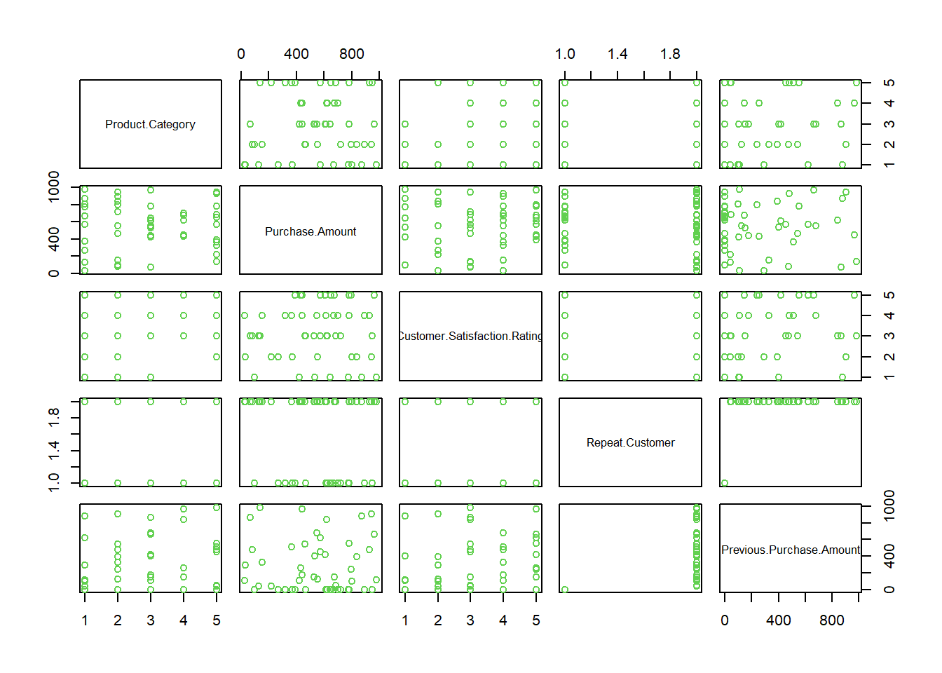
13.10 Correlations?
plot(Purchase.Amount ~ Previous.Purchase.Amount,
     data=customer_sales, col="blue")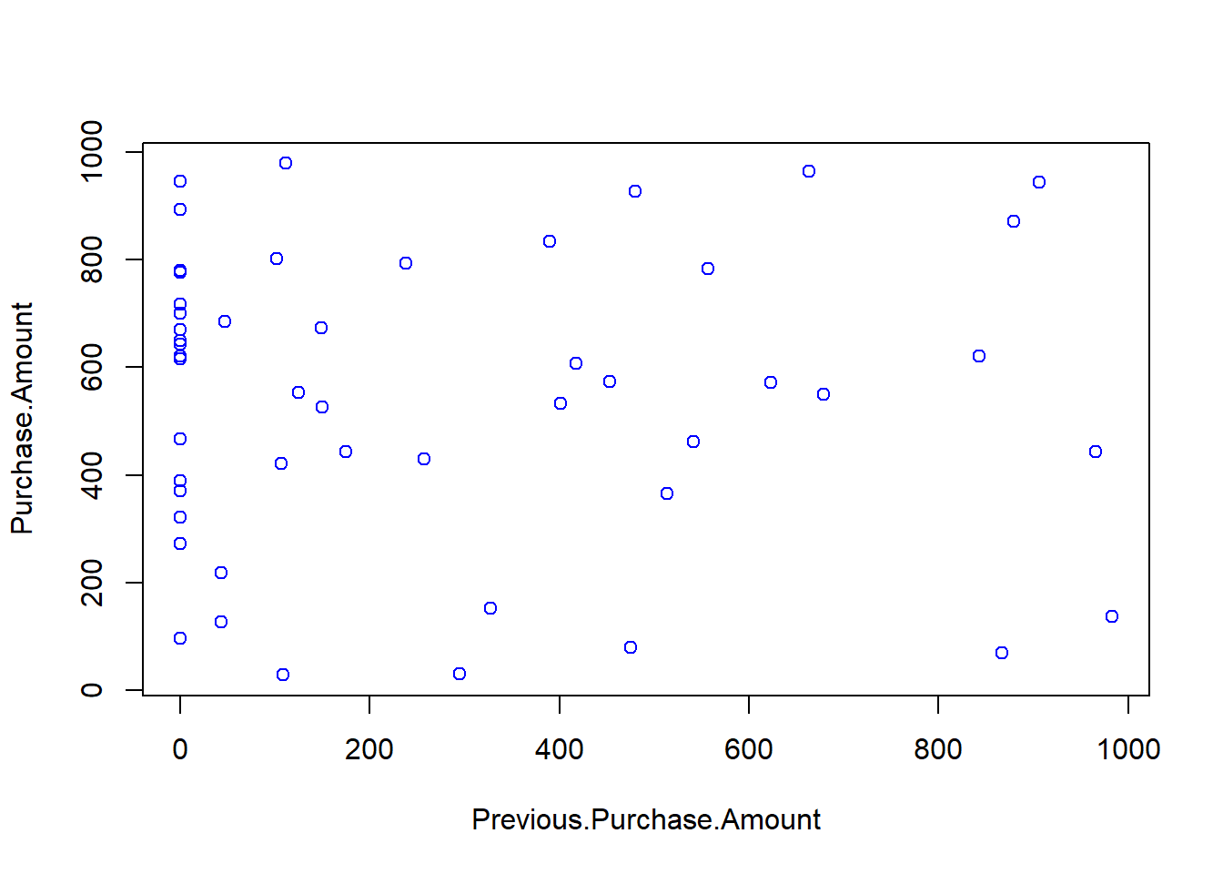
13.11 Graphical parameters
Search for more features to customize your plots by typing:
> ?plot
> ?points
> ?par
For colour palettes in base R plots use:
> palette()
Example:
plot(Purchase.Amount ~ Previous.Purchase.Amount,
     data=customer_sales, col="blue", pch=19)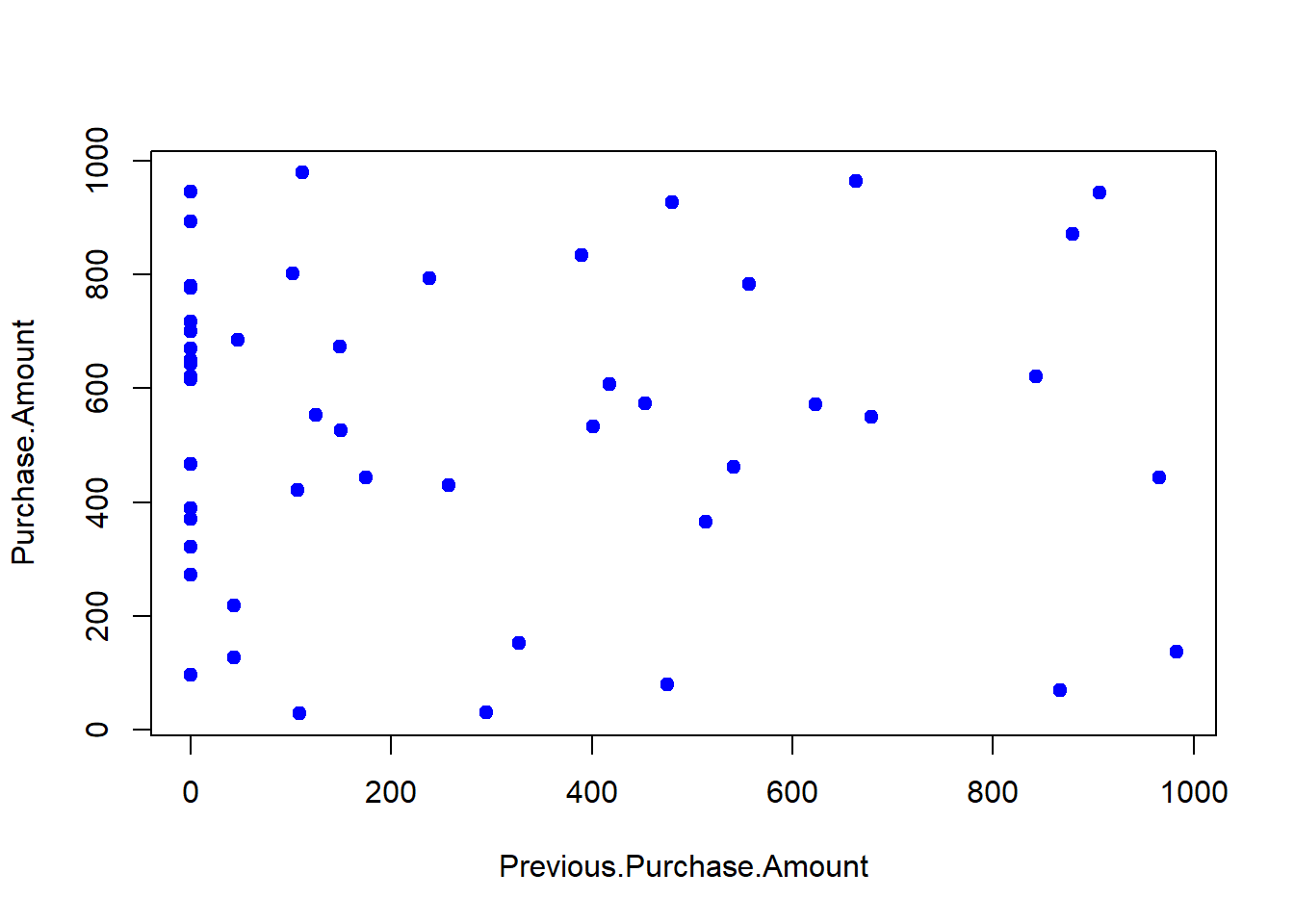
13.12 Reflection questions
Reflection Questions
What could go wrong if the top row of your spreadsheet doesn’t contain variable names?
What does the dim() function tell you about your dataset? Why is it useful?
How do packages like dplyr enhance the data analysis process compared to using base R?
Why do you need to run library(“dplyr”) each time you start a new R session, even if the package is already installed?
How does chaining functions with the pipe %>% make your code easier to read?
What insights can you gain by creating a scatterplot matrix of your dataset?
What is one new graphical customization you discovered using the ?plot, ?par, or ?points help pages?
13.13 Exercises
Exercises
What is the goal of the dplyr package, and why do many analysts prefer it over base R for data manipulation?
Why might you choose to use filter() over using logical indexing directly in base R?
What makes mutate() particularly useful when working with grouped data?
What is the main difference between mutate() and summarize()?
Why is arrange() combined with desc() often used in practice?
Why might you choose to use select() instead of subsetting columns with [ , ] in base R?
Explain the relationship between group_by() and summarize(). Why does group_by() not change the dataset on its own?
What problem do tibbles solve compared to base data frames?
How does the pipe operator %>% change the way you write and read code?
For questions 10 to 15, use the following dataframe:
orders <- data.frame(
  order_id = 1:5,
  customer = c("A","B","C","D","E"),
  year     = c(2025,2025,2024,2025,2024),
  total    = c(200, 1200, 450, 800, 300),
  discount = c(20, 100, 0, 50, 10)
)
Keep only the columns order_id, customer, and total using select() with the pipe operator.
Filter to show only rows where total > 500 and year == 2025.
Add a new column called net to orders that equals total - discount. Use mutate().
Sort the orders dataset by total in descending order. Use arrange() with desc().
Group the orders dataset by year and compute the average order total in each year.
Karl wrote:
orders <- select(order_id, customer, total) %>% ordersCorrect the code.
Explain what a tibble is. Convert the orders dataset into a tibble and observe how it prints differently compared to a data frame.
Explain what the pipe operator %>% does. Rewrite this nested call using the pipe:
summarize(group_by(orders, year), avg_total = mean(total))What is the advantage of a scatterplot matrix over looking at pairs of plots individually?
Why is it important to learn how to add parameters like points(), par(), and color palettes to plots?
How could adding the pch (point character) parameter help when creating scatterplot matrices with groups of data?
For questions 21 to 28, use the built-in dataset mtcars.
Create scatterplots of mpg vs hp and mpg vs wt in a single window using par(mfrow=) and the plot() function.
Filter rows where mpg > 25 OR hp < 100. Write the code using filter().
Plot mpg against wt using formula notation (y ~ x). Add labels for the axes and a title.
Highlight 6-cylinder cars in the above scatterplot by adding points with a different symbol and size.
Color points in the mpg ~ wt plot by cylinder group (4, 6, 8) using a custom palette.
Add two new variables to mtcars:
- power_to_weight = hp / wt
- kpl = mpg / 2.35 (to convert miles per gallon to kilometers per liter)
Group by cyl and calculate both the average mpg and the maximum hp for each group.
Rewrite this nested call using the pipe operator:
head(arrange(filter(mtcars, mpg > 20), desc(hp)), 5)- Why does the formula interface (y ~ x) in base R plotting make code more robust?